Package this!

R packaging and all that.

I've been having a few problems building/checking a package in Rstudio and have been writing this so I don't suffer again. I haven't added anything to my blogger site in ages, because blogdown has taken over my technical blogging - but, since this post will involve making a package from scratch using the Rstudio witchcraft and it isn't obvious how package-creation could be done and documented within an Rmarkdown file, I'm just going to post screenshots here (and eventually move the figures over to blogdown)

This blogpost is errors included. Hopefully I'll end up with a cleaner package-setup workflow and include a TL/DR to summarise that. But I like to see where people ballsed-up and how they learned, and learning programming typically involves a lot of the former...

----

Create a new environment (under miniconda using conda-forge)

conda create --name pkg_temp -c conda-forge \

    r-base=3.5.1 r-devtools=2.0.1 r-roxygen=6.1.1

conda activate pkg_temp

conda install rstudio=1.1.456

Start Rstudio

rstudio &

----

Create a new package

Within Rstudio:

File ->

  New Project ->

  [Create Project within a] New Directory ->

  [Project Type is an] R Package -> ...

We set the package name to be "hello_world", then "new_project", then "temp_project". In each case the text-entry field went red.

It went red, because it doesn't want underscores in the package name.

So we set the package name to be "helloProject"; this adds a new subdirectory to the file system. We didn't add .git, use any existing source files or use packrat

The package is initialised with a "hello.R" file (this appears to be the default for new packages in Rstudio).

----

Get that initial package to pass `devtools::check()`

`devtools`, `usethis` and `roxygen2` are the (current) standard tools for assisting you make and document packages in R.

I loaded `devtools`, `usethis` and `roxygen2` so that they are available within the console in Rstudio, although they are implicitly available: you can build / install / test a package from the Build tab in Rstudio [in the top-right of the image below (your build tab may be elsewhere)].

We have the skeleton of a package. The package contains a single function (`hello`). Let's see what we need to do to get that package installable:

Nothing! We just clicked "Install and Restart" and the template package installed (we could similarly have used `devtools::install()` in the console).

But. If you want to release a package you have to get your package to pass R's package "check"ing workflow. At the command line you'd write `R CMD check <my_package...>`, in the console you'd use `devtools::check()` and in Rstudio you'd use `Build -> Check` or [Ctrl-Shift-E] (or similar; shortcuts are written for the linux version of Rstudio). Using `Build -> Check` on the template package we get the following:

[Choosing a license]

`Check` failed because we have yet to pick a license. 

The DESCRIPTION file holds a variety of info about your package. Before we choose a license it looks like this:

I usually use the MIT license. To choose this using the console we do this:

usethis::use_mit_license(name = "My Name")

That didn't fail, but it looks like it wasn't happy (we have some warnings related to the contents of the DESCRIPTION file, but can ignore them). The DESCRIPTION now looks like this (and a couple of files called LICENSE and LICENSE.md have been added to the root directory):

We'll check the package again:

So that all seems great. We have a package containing a single function, it can be installed and it passes the checks.

----

Ensure we can update the package docs & code

The template package had an `R/hello.R` (the source code) and a `man/hello.Rd` file (the documentation for that source code). The contents look like this:

[R/hello.R]

[man/hello.Rd]

Let's change that hello.R file so that it returns a data.frame with "hello" in one column and "world" in another The code in `hello.R` now looks like:

hello <- function(){

  data.frame(x = "hello", y = "world")

}

We install and check the package (both are fine). Calling `hello()` returns a data.frame but when we call `? hello` it says the function _prints_ out "Hello, world!", so the documentation is out of sync with the code.

We could modify "man/hello.Rd" to reflect the change to the `hello` function. But by using `roxygen2` we can have the content for the documentation for `hello` stored with the source code (ie in R/hello.R), and have the documentation-files that R uses (ie, man/hello.Rd) generated automatically from the source code. This simplifies development a bit. 

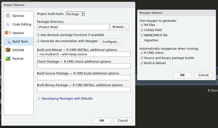
`roxygen2` is available in our environment (see the conda stuff, above). To use it within this project, we have to tell Rstudio that we want to use `roxygen2` to generate the `*.Rd` documentation files whenever we build our package. To do this, go through `Tools -> Project Options -> Build Tools` and click "Generate documentation with roxygen" (and then click Automatically roxygenize when running "Build and reload" in addition to the existing options)

Now we can update the docs from the definition of the `hello` function within the source file `R/hello.R`.

When generating documentation with roxygen, typically you would build/install the package (with [Ctrl-Shift-B] or `Build -> Install and Restart`) or use [Ctrl-Shift-D] or `Build -> More -> Document`. In a package, `roxygen2` would then create any of the `man/*.Rd` files and update the `NAMESPACE` file (the latter indicates which packages / functions / classes are to be imported-into or exported-from the current package).

We can't do that yet. If any of the files that `roxygen2` wants to make are already in existence (and haven't been made by roxygen itself) it won't make those files. So, since `hello.Rd` and `NAMESPACE` already exist in our skeleton package, these won't be automatically made. Running the roxygen2-Documentation workflow ([ctrl-shift-D]) gives the following in our project:

Indeed, if we reload our package and call `? hello`, the help-page shows that hello should print, but it returns a data.frame.

So, we delete the existing `man/hello.Rd` and `NAMESPACE` files and rerun roxygen2-Document. It works this time:

[Ctrl-Shift-D - after deleting the existing files]

We reinstalled the package [Ctrl-Shift-B] and checked the function / help-page:

Well that's pretty weird. The function can't be called now, but the documentation can be read. The problem is that we haven't exported the function.

The original NAMESPACE file contained a rule that exported anything found in files of the form "R/*.R". But we're now using roxygen2 to both generate the documentation (which it's done) and the NAMESPACE file (which it has done, but it isn't quite how we wanted it). Aside from a comment, the NAMESPACE file is empty at the moment:

To ensure that our `hello` function is exported, you could modify NAMESPACE (adding the line `export(hello)`); but that comment is warning you not to make any changes to it. To ensure `hello` is exported, you add an `@export` roxygen annotation to the `hello`-function's docstring:

We can reinstall the package (and automatically update the NAMESPACE & documentation, since roxygen2 is now ran everytime we build the package, see above) and `hello()` should be available.

[Ctrl-Shift-B]

----

Import a function from another package (without using it)

Now that we can install, check and automatically document a package, let's break it on purpose.

We use the `roxygen2` `@importFrom` annotations to make external functions available in our new package. Suppose that, rather than using `data.frame` we wanted to use `data_frame` from the `tibble` package. There are several reasons for preferring the latter: `data_frame` doesn't automatically convert strings to factors, the returned objects have nicer default printing behaviour and it doesn't bork up your column names.

We add an `@importFrom` annotation to import `data_frame` from `tibble` and replace the call to `data.frame` with `data_frame`:

Then we document/build/reinstall (no problems), and check [Ctrl-Shift-E]. Check failed with an error "Namespace dependency not required: `tibble`".

We are trying to use a function from an external package (tibble) within our local package (helloPackage). Suppose R is loading our package into a new session, how does it know which external packages must be available, and which packages/functions to import? It looks in DESCRIPTION and NAMESPACE.

DESCRIPTION tells R which packages are required for our package to work (in addition to authorship and licensing information). During a call to `install.packages` these external packages will be installed prior to installation of our package.

NAMESPACE tells R which functions to import from those packages or, which packages to import wholesale (and explains which functions are exported from our package)

So to use the `tibble` package, we should have updated DESCRIPTION and NAMESPACE. roxygen2 updates NAMESPACE automatically - as we can see in the current NAMESPACE below:

But DESCRIPTION hasn't been updated to say that our package depends upon tibble. We shouldn't try to use a function from an external package if we can't be certain that that external package is available in the environment where we are trying to use our package.

We can update DESCRIPTION by hand, or use `usethis::use_package` to ensure that R knows that `tibble` is a prerequisite for our package. We prefer the latter since it's less prone to typos. `data_frame` was first exported from version 1.0.0 of `tibble`, and from version 1.5.0 of `usethis` we can specify a minimum-version of an external package for use within a package we are developing -

After a call to:

usethis::use_package(
    "tibble",
    # with usethis >= 1.5.0 we can specify a minimum version:
    min_version = "1.0.0"
)

... our DESCRIPTION looks like this (note the format for specifying the minimum package versions):

We now document / build / install [Ctrl-Shift-B] and Check [Ctrl-Shift-E]: all pass without any issues.

----

[TODO: Pass the barebones package through styler, lintr and get it to pass all goodpractice checks (except cyclocomp)]

[TODO: Add github repo; Do the minimal to set up and pass travis integration]

----
ACK! `data_frame` is being withdrawn from `tibble` so the example running through this post is already bad practice (I could rewrite using `tibble::tibble` but that would lead to a confusion between the name of the external-package and the name of the function imported from that package)

reporters in testthat

(2018-04-24): testtthat authors don't currently have a vignette re the different reporters used by testthat.

I'm currently trying to work out how best to use these reporters in a shell script that runs my tests.

To use a reporter using testthat or devtools your code looks like this:

devtools::test(my_dir, reporter = CheckReporter)

or equivalently

testthat::test_dir(my_dir, reporter = CheckReporter)

They reporter can also be defined as a string: the string corresponding to CheckReporter being "check"

`CheckReporter` and the other *Reporters are imported into your namespace as objects. you don't need to instantiate them `new("CheckReporter")`  or call them `CheckReporter()`.

For non-interactive use the appropriate reporters are:

CheckReporter, FailReporter, JUnitReporter, ListReporter,  TapReporter, TeamcityReporter

For interactive use the appropriate reporters are:

DebugReporter, LocationReporter, MinimalReporter, ProgressReporter, RstudioReporter, SilentReporter, StopReporter, SummaryReporter

MultiReporter is used for combining results together

----

I find SummaryReporter the simplest to use when using R interactively.

TO BE FINISHED

----

Summaries of  the available testthat reporter objects from within the testthat pdf

CheckReporter
R CMD check displays only the last 13 lines of the result, so this report is design to ensure that you see something useful there.

DebugReporter
This reporter will call a modified version of recover() on all broken expectations.

FailReporter
This reporter will simply throw an error if any of the tests failed. It is best combined with another reporter, such as the SummaryReporter.

JunitReporter
This reporter includes detailed results about each test and summaries, written to a file (or stdout) in jUnit XML format. This can be read by the Jenkins Continuous Integration System to report on a dashboard etc. Requires the xml2 package.

ListReporter
This reporter gathers all results, adding additional information such as test elapsed time, and test filename if available. Very useful for reporting.

LocationReporter
This reporter simply prints the location of every expectation and error. This is useful if you’re trying to figure out the source of a segfault, or you want to figure out which code triggers a C/C++ breakpoint

MinimalReporter
The minimal test reporter provides the absolutely minimum amount of information: whether each expectation has succeeded, failed or experienced an error. If you want to find out what the failures and errors actually were, you’ll need to run a more informative test reporter.

MultiReporter
This reporter is useful to use several reporters at the same time, e.g. adding a custom reporter without removing the current one.

ProgressReporter
This reporter is a reimagining of SummaryReporter desgined to make the most information available up front, while taking up less space overall. It is the default reporting reporter used by test_dir() and test_file().

RstudioReporter
This reporter is designed for output to RStudio. It produces results in any easily parsed form

SilentReporter
This reporter quietly runs all tests, simply gathering all expectations. This is helpful for programmatically inspecting errors after a test run. You can retrieve the results with the expectations() method.

StopReporter
The default reporter, executed when expect_that is run interactively. It responds by stop()ping on failures and doing nothing otherwise. This will ensure that a failing test will raise an error.

SummaryReporter
This is a reporter designed for interactive usage: it lets you know which tests have run successfully and as well as fully reporting information about failures and errors.

TapReporter
This reporter will output results in the Test Anything Protocol (TAP), a simple text-based interface between testing modules in a test harness. For more information about TAP, see http://testanything.org

TeamcityReporter
This reporter will output results in the Teamcity message format. For more information about Teamcity messages, see http://confluence.jetbrains.com/display/TCD7/Build+Script+Interaction+with+TeamCity

vimpressive things

vim things

----

Run a shell script/command over the current file

:! <command_name> %

eg, get the number of lines in the current file:

:! wc -l %

----

Count words in selection
In visual mode: g Ctrl-g

----

Reload the current file
In normal mode:  :e

----

a few of my favouRite things

2018-05-04

Matrix::Matrix

See here and here

Matrix provides sparse-matrix objects to R. So if you're making matrices that are mostly zero use `Matrix` not `matrix`.

I recently used Matrix while trying to work out the overlap sizes between a few hundred different sets of genes. The genesets were represented as a list of vectors of gene-ids; each vector being a single geneset. My initial code `map`ped over the collection of genesets twice, to pull out each pair of genesets, and then compared the intersection sizes of the two genesets.

THIS TOOK FOREVER!

So, instead for the G genes and the S genesets, I made a sparse G x S binary matrix, where the i,j'th entry indicated whether gene i was present in geneset j. In graph theory language, this is a biadjacency matrix over a bipartite graph, wherein the edges represent the presence of a gene in a geneset and there is a node for each gene and each geneset.

Let M be that matrix. We can construct it as follows:

make_biadjacency_from_list <- function(
    genesets,
    universe = NULL
  ) {

  if (is.null(universe)) {
    universe <- genesets %>%
      purrr::reduce(union) %>%
      sort()

    }

  incidence <- Matrix::Matrix(
    0,
    nrow = length(universe),
    ncol = length(genesets),
    sparse = TRUE
  ) %>%
    magrittr::set_rownames(universe)

  for (j in seq_along(genesets)) {
    genes <- genesets[[j]]
    rows <- which(universe %in% genes)
    incidence[rows, j] <- 1
  }
  incidence
}

M <- make_biadjacency_from_list(my_gene_sets, my_gene_universe)

That runs in seconds. Then the geneset overlap sizes can be pulled out from t(M) %*% M since the i,j entry of this matrix is the number of genes present in both geneset i and geneset j.

get_overlap_counts <- function(
    biadj
  ) {
  # determine the overlap counts by taking the inner product
  # - note that codegree is a Matrix provided `biadj` is one
  codegree <- t(biadj) %*% biadj

  # the diagonal elements define the number of genes in each
  # geneset
  set_sizes <- diag(codegree)
    
  # identify indices for pairs of genesets with non-zero overlap,
  # refer to them as set1 and set2
  overlapping_sets <- 
    which(as.matrix(codegree) != 0, arr.ind = TRUE) %>%
    as_data_frame() %>%
    set_colnames(c("set1", "set2")) %>%
    filter(set1 != set2)

  # add the geneset overlaps and the sizes of both set1 and set2
  # - note the pattern for vectorised extraction from a Matrix
  # - codegree[set1, set2] would return a subMatrix not a vector
  overlapping_sets %>%
    mutate(
      set1_size = set_sizes[set1],
      set2_size = set_sizes[set2],
      set_overlap = codegree[cbind(set1, set2)]
    ) %>%
    mutate_all(as.integer)
}

Then I ran my fisher tests using the geneset sizes and overlap sizes returned by get_overlap_counts(M).

Thank you, sparseness.


2018-05-02

tidyr::nest

See here and here

In dplyr, I often want to group-by some columns, apply a function to the subtables defined by grouping, and then dissolve away the group-by.
The function applied to the subtables may return

- a single row for each group: in which case you'd use dplyr::summarise() or summarize()
- a row for each row in the subtable: in which case there may be an appropriate window function
- any number of rows for each subtable

In the latter case, you want to use tidyr::nest()

Suppose I've got a data-frame with gene-expression data for three different tissues. The columns are "tissue", "gene_id" and "expression". For each tissue, I want to find the top-10 most highly expressed genes (according to the value of expression).

df <- tibble(
  tissue = rep(LETTERS[1:3], each = 26),
  gene_id = rep(letters, 3),
  expression = rnorm(78)
)

The following function would extract the top-10s for a given tissue if there was only one tissue in the dataframe

get_top10 <- function(.df){
  arrange(.df, desc(expression)) %>%
    head(10)
}

I could `split` the data-frame into a list based on the "tissue" values, order the subtables by expression, take the head of those subtables and join them back up. Something like

df %>% 
  split(f = df$tissue) %>% 
  map_df(get_top10)

Which works perfectly fine.

Or, I could use nest

df %>%
  group_by(tissue) %>%
  nest() %>%
  mutate(data = map(data, get_top10)) %>%
  unnest()

The value of nest() over split() is that you can group_by multiple different columns at the same time and you don't have to do that ugly df$my_column stuff.


2018-03-29

knit_expand

- If anyone reading this is aware of a way to use knit_expand to include a dynamic number of figures in the same way as the following (for tables), please comment -

Rmarkdown is great. It's lightweight and it's versatile; compared with .lyx and jupyter-notebooks it doesn't surround your code with tag-crap and it's consequently easier on git (and you don't get an equivalent of `pushed-a-compiled-ipynb-to-bitbucket` hell).

But sometimes you need to know little tricks.

You can only print a single result from a given R code-block. And sometimes you want to print out the same `kind` of result multiple times.  For example, you might have ran 8 analyses and want to print out a table for each analysis.

Pffft, just write my_tables[[1]], my_tables[[2]], .... my_tables[[8]] in 8 different blocks - DONE!.... ?

That's some ugly stuff going on right there. What if you add another analysis. What if you want to subfilter each table. What if you want to do XXX that means you'll have to touch each of those 8 lines of code or add an extra identical line of code?

Use `knit_expand` inside a map and then knit the result - this formats your code ready for printing . Each call to knit_expand will convert your code to a knittable form.

```{r}
out <- purrr::map_chr(
  my_tables,
  function(tt){
    TT <- modify_my_table(tt)
    knit_expand(text = "{{TT}}")
  }
)
```

`out` now contains a few different tables. It's contents will be printed when the current .Rmd document is compiled if you put the following where you want the tables outputting:

`r paste(knit(text = out), collapse = "\n")`

So you don't have to write a separate block for each table.


2018-03-26

map an extraction

I can't believe I only just found this out, considering I've been using `purrr` for a while. I often have to map over a list of identically structured elements, and extract a subcomponent of those elements.

Suppose you want to extract the 'y' element of each element of the following list into a separate list

# input:
my_list <- list(
  a = list(x = 123, y = 234),
  b = list(x = 567, y = 789)
)
# intended output:
# list(a = 234, b = 789)

Here's how I'd have done it:
purrr::map(my_list, function(z) extract2(z, "y"))
# or
purrr::map(my_list, function(z) z[["y"]])

Then you end up doing this stuff quite often, and so you write a shortcut, but it's ugly because you can't easily partialise `extract2` or `[[`

map_extract2 <- function(xs, i){
  map(xs, function(x) extract2(x, i))
}

ys <- map_extract2(my_list, "y")

Then you think: `this is stupid, surely there's already a shortcut for this!`

There is, and its' dead simple.

ys <- purrr::map(my_list, "y")

*Bangs head*


2018-03-02

styler / lintr

Your code makes me wince; so does my right-brain's code. Get it pretty, stat!.

My R code now looks like this (as of 2018):
ClassName
object_name / column_name
verb_prefixed_function_name
.non_exported_function_name

Regarding stuff like

• '<-' vs '=' (walk with the idiomatic former);
• column/parenthesis alignment (pfft);
• double- vs single-quotes (arbitrarily choose the former);
• superfluosity of whitespace (yes around args, no at the end of lines); 
• keeping your code in a scannable page width

... I do care about this sort of stuff but not while I'm writing.

1. `styler` catches some of these things and automatically alters them to an approximation of tidyR style; 
2. and some things that you wouldn't trust automated tools to alter can be indicated by `lintr`. 

I mostly write within vim and `lintr` can be set up to run automatically every time you save and I have a shell script to call `styler` on the current file.

When I'm writing in Rstudio, styler can be ran from the `Addins` and lintr from the console (lintr works great for packages in Rstudio, but is a bit of a chore to set up which linters to use for a general analysis project vs in vim, IMO).

I've also a script that fixes my roxygen comments for questionable and finicky reasons.

And all three tools are being pushed into a git hook that runs over all R/Rmd files prior to commit.

2018-02-21

ggplot2::`%+%`

Although it's mostly related to the objects-first languages that I rarely use, I've been reading Refactoring by Martin Fowler. In this book they defined a number of `code smells` - signals of underlying filth in your programs. Deep within that dognest lies "Duplicated Code" - a smell that is far-from restricted to OO programming. So I wrote a little function to find duplicated code in my R scripts (because I couldn't find a good package to do that - if you know of one pleeease comment) and let it run.

BANG! The main source of duplicated code in my scripts was ggplot2 calls of the form:

data %>% filter %>% define_aesthetics + define_geoms + format

Sometimes the first half of the call was duplicated, and sometimes the latter.

If you find yourself writing the same

define_aesthetics + define_geoms + format

steps over and over, use ggplot2::%+% instead.

my_df <- data_frame(a = 1:6, b = rep(letters[1:2], each = 3))
my_df %>% filter(b == "a") %>% ggplot(aes(x = a)) + geom_density()
my_df %>% filter(b == "b") %>% ggplot(aes(x = a)) + geom_density()

Rethink that duplicated code:

# define the graph for the first subset
p <- my_df %>% 
     filter(b == "a") %>% ggplot(aes(x = a)) + geom_density()

# plot the data for the first subset:
p
# plot the data for the second subset by replacing the data used by ggplot2
p %+% filter(my_df, b == "b")

[Admittedly that was a simple example, and has better solutions using faceting]


2018-02-20

gtools::mixedsort

Converting strings that contain numbers into factors and wondering why G10 comes between G1 and G2? That's because '10' is alphabetically-lower than '2'. To fix this, you can either specify your factor levels explicitly, or you can let `mixedsort` do it for you.

# Que?
paste0("G", 1:10) %>% factor()
# [1] G1 G2 G3 G4 G5 G6 G7 G8 G9 G10
# Levels: G1 G10 G2 G3 G4 G5 G6 G7 G8 G9

# But check this:
library(gtools)
paste0("G", 1:10) %>% factor(levels = mixedsort(.))
# [1] G1 G2 G3 ... G10
# Levels: G1 G2 G3 G4 G5 G6 G7 G8 G9 G10

I tend to use a wrapped function to do this.

factor_mixedsort <- function(x){
  factor(x, levels = gtools::mixedsort(unique(x)))
  }

so that I can use a single function call when I'm making plots etc


META
Some things are so unequivocally in my favouRite things, and are so widely known, that I haven't written about them:
%>%
roxygen2
rmarkdown
testthat


TODO
- here (again)
- filter_at & friends
- stringr::str_interp (vs paste / sprintf)
- suppressPackageStartupMessages / suppressMessages
- the `eval` flag in Rmarkdown chunks
- tidyr::unite


ASIDES
Here are some other peoples favourite things:
- some simple rstudio tips


THE CONTINUALLY UPDATED LIST OF THINGS I WANT TO LEARN
Here are some things that might one day make it into my favourite things:
- Hmisc::escapeRegex
- brms
- future
- patchwork (vs cowplot / arrangeGrob)
- tailr
- tabr
- TBC

Regression lines in ggplot

Based on a question at today's code-club, here's how you plot a scatter plot with an overlain regression line in ggplot2:

Set up some data and import the necessaries:

library(tibble)
library(ggplot2)

set.seed(1)

x <- rnorm(30)
y <- rnorm(30, x)
my_df <- data_frame(x = x, y = y)

Here, x and y are sampled from a normal distribution and the expected slope of the regression line of y on x is 1.

A scatter plot of y against x is as follows:

gg <- ggplot(my_df, aes(x = x, y = y)) +
  geom_point()

gg

If you're happy for R to compute the appropriate regression line for you, you can use the following to overlay the line:

gg + geom_smooth(method = "lm", se = FALSE)

Otherwise, you can compute the parameters of any line that you want to include, and then overlay them using geom_abline.

To do this, we first calculate the regression coefficients for y against x

fit <- lm(y ~ x)
coef(fit)
# (Intercept)         x
#    0.129...   1.04...

.. and then overlay the associated linegraph (we've used col = #3366FF to match the defaults for GeomSmooth)

gg +
  geom_abline(
    intercept = coef(fit)["(Intercept)"],
    slope = coef(fit)["x"],
    col = "#3366FF"
    )

You can pick your own slopes / intercepts.

Pushing r-eulerr onto anaconda using conda-skeleton / conda-build / anaconda-upload

CRAN package eulerr is not available on anaconda as of 2018/01/19. I have other blogs that include notes on how to upload packages to anaconda, but they're a bit scruffy. Here's another neater version.

In my root conda environment I first updated conda and python
conda update conda
conda update python

and then did:

cd ~/tools/conda_recipes
conda skeleton cran eulerr
conda build --R=3.3.2 r-eulerr

# dependency r-rcppde is missing:

conda skeleton cran RcppDE
conda build --R=3.3.2 r-rcppde

# Failed with warning:
/usr/bin/ld: cannot find -lgfortran

# Installed gfortran (but somewhat dumbfounded that it wasn't already present)
sudo apt-get install gfortran

conda build --R=3.3.2 r-rcppde

anaconda upload ~/tools/miniconda3/conda-bld/linux-64/r-rcppde-0.1.5-r332hf484d3e_0.tar.bz2

conda build --R=3.3.2 r-eulerr

# Failed
Error: package ‘Rcpp’ 0.12.8 was found, but >= 0.12.12 is required by ‘.’

# Changed meta.yaml for r-eulerr to say
host:
  - r-rcpp >=0.12.12
  ...
run:
  - r-rcpp >=0.12.12
  ...

conda build --R=3.3.2 r-eulerr

anaconda upload ~/tools/miniconda3/conda-bld/linux-64/r-eulerr-3.1.0-r332hf484d3e_0.tar.bz2

DONE!

upsetR plots

Venn diagrams blow. 
Multiset Venn diagrams both blow and suck:

• Don't make them;
•  and don't make me interpret them;
•  and don't try and put them in your presentations because you'll get lost

UpSetR provides a way to do the multi-set comparison thing without looking horrific.

We sample a few sets from the letters `b-z`:

library("UpSetR")

set.seed(1)

bucket_names <- paste0("set", 1:6)

buckets <- Map(
  function(x){
    bucket_size <- sample(1:25, 1)
    bucket <- sample(letters[-1], bucket_size, replace = FALSE)
    },
  bucket_names
  )

lapply(buckets, sort)
$set1
[1] "f" "k" "n" "o" "t" "v" "x"

$set2
 [1] "c" "d" "f" "h" "i" "j" "k" "m" "n" "o" "q" "r" "s" "w" "y" "z"

$set3
 [1] "b" "e" "i" "k" "l" "m" "p" "v" "x" "y"

$set4
 [1] "b" "c" "d" "f" "g" "i" "k" "l" "n" "o" "p" "q" "s" "t" "u" "v" "w" "x" "y"
[20] "z"

$set5
 [1] "c" "f" "h" "j" "k" "n" "q" "r" "s" "t" "v" "w" "y"

$set6
 [1] "b" "c" "d" "e" "f" "g" "i" "j" "k" "l" "m" "n" "p" "q" "r" "s" "t" "u" "w"
[20] "x" "z"

The function `upset` takes a dataframe as input. But I've just defined my sets as a list of vectors. To convert these into a dataframe, use `UpSetR::fromList`:

fromList(buckets)

   set1 set2 set3 set4 set5 set6

1     1    1    1    1    1    1

2     1    1    0    1    0    0

3     1    0    1    1    1    0

4     1    1    0    1    1    1

5     1    0    0    1    1    1

6     1    0    1    1    0    1

7     1    1    0    1    1    1

8     0    1    0    1    1    1

9     0    1    1    1    1    0

10    0    1    0    1    1    1

11    0    1    0    0    1    1

12    0    1    0    1    1    1

13    0    1    0    0    1    1

14    0    1    0    0    1    0

15    0    1    1    0    0    1

16    0    1    0    1    0    1

17    0    1    1    1    0    1

18    0    1    0    1    0    1

19    0    1    0    1    1    1

20    0    0    1    1    0    1

21    0    0    1    1    0    1

22    0    0    1    0    0    1

23    0    0    1    1    0    1

24    0    0    0    1    0    1

25    0    0    0    1    0    1

The letter 'a' is absent from every one of these sets. you could add a `universe` entry or a `unobserved` entry to the set-list passed to `fromList` if that's what you're into.

Otherwise, to generate an upset plot do the following:

upset(
  fromList(buckets)

  )

This gives the following plot:

We note a couple of things: 

• `set1` is absent from the image, although it contained 7 elements;
• the elements of a given set are partitioned between the bars: eg, `set3` contains 9 elements, that are split over the 4-5th, 8-9th and 12-14th columns (the numbers above these columns add up to 9) so each element in set3 is put into a single column
• that means, although the intersection between set3 and set6 is of size 8, there is only one element in the "set3 and set6" intersection column (the remaining 6 are partitioned across the other columns that contain both set3 and set6)

To ensure that all the sets are displayed in the figure, modify the `nsets` argument:

You can order the bars by size (`order.by = "freq"`) or by the number of sets that contributed to the intersection (`order.by = "degree"`) or by both:

# order by freq
upset(
  fromList(buckets), nsets = length(buckets), order.by = "freq"

)

# order by degree and then by freq (not shown)
upset(
  fromList(buckets), order.by = c("freq", "degree"),
  nsets = length(buckets)
  )
# order by freq and then by degree (not shown)
upset(
  fromList(buckets), order.by = c("degree", "freq"),
  nsets = length(buckets)

  )

I found the latter a bit weird, in that order.by = c("degree", "freq") sorts by increasing frequency, whereas order.by="freq" sorts by decreasing frequency.

That'll do