biolearnr: Start playing with R and Bioconductor

Eloquent introductions are hard to write

Best thing to do is just start playing

If you've never programmed before, learning R will be as difficult as learning any other language. And here we assume you've never programmed before. This post isn't about making you a programmer though, it's about doing biology in R. We're eventually going to use bioconductor to analyse some microarray data, but, before we do that you'll need to have R installed and some understanding of syntax and structure. This will be something of a whirlwind tour, some bits will seem unnecessary, but I'll try to tie everything into microarray analysis. There are many, better, introductions to R and bioconductor, literally everywhere on the web.

As with all coding tutorials:

type it in yourself
modify it
read around it
save it in a script
explain it back to yourself in comments

As with all data analysis:

Think how you'd do it with just a calculator
Think how you'd do it in an ideal world
Work out why they don't do it the way you (or some book) would suggest
Try it on something new
Try it on something randomised
Watch out for broken symmetries
Watch out for biases
Watch out for arbitrariness

Installing R

The easiest way to install R is to follow the install instructions for RStudio.

You can obtain R from here

follow the links through "Download R for [Windows|Linux|OsX]"
run the .exe or the .pkg or whatever
agree to the various things in the setup
once you've downloaded and installed it, run R from it's icon (or from the command-line on linux).

This is the base front-end for R, and it's a barren, barren place - fortunately we won't be spending any time here. You could type in demo("graphics") into the prompt to see some example graphs that could be made in R. You can make way cooler graphs that these examples, though - have a look at the R-Graph-Gallery.

Then you can install RStudio-Desktop afterwards for free from here (again just download and run the installer).

RStudio runs on windows/mac/linux and provides a neater front-end to the R language than basic R does. On running the program it provides 4 windows:

the R console (where you can interactively type in R commands; bottom left);
a text editor for writing scripts (keeping your analysis in a script makes it easier to rerun an analysis on a different day, or using different data, so please <!!> write your work up in a script; top left - this panel might not be visible when you first open RStudio, if it isn't clickthrough File->NewFile->RScript);
a window that stores info about all the data that R is currently working with (variable names etc; top right); and
a window that stores a variety of other house-keeping things - what files are in the current directory, what figures have you made during the current session, what packages (that is, extensions to the R language) you've got loaded (bottom right).

[I don't actually use RStudio though - I typically write R code in jupyter notebooks (which combines interactive and scripting work), in the text-editor vim (when I'm working on packages and scripts) and in lyx (when I'm writing formal reports); and for reproducibility's sake use anaconda/bioconda to control which release of R and it's packages that I use for any given project]

Variables, values and functions

R was originally a language for statistical computing. Anything you'd need for analysing and presenting data has already been written, it's just a case of piecing those things together. First you need to store some data in a variable and we can get cracking.

# This is a comment since it follows a '#' character

# In the following: `a` is the name of a variable

# : 123 is the value stored in the variable `a`

# : `<-` assigns the value 123 to the variable a

a <- 123

There is a range of different types of value that can be stored in a variable. These include simple things like numeric values (123, NaN, Inf, 6.022e23), string values ("hello world"), boolean values (TRUE, FALSE), factors (effectively categorical variables; more later) or the bizarre value of nothingness: NULL. More complicated datatypes include vectors, matrices, lists and data.frames.

Vectors

Vectors are a 1-dimensional collection of values of a particular type (so, a given vector can't contain both numeric values and string values for example). We can build a vector using the function c() or by using some other built-in tools, since a lot of R's functions return vectors. Note that vectors can contain at most -1 + 2^32 ~ 4*10^9 entries - which sounds like a lot - unless you work with a genome containing 3 billion letters.

vector.of.integers <- c(1, 3, 7, 8)
vector.of.strings <- c("hello", "world")
vector.of.booleans <- c(TRUE, FALSE, F, T, FALSE, TRUE)

vector.of.floatingpoints <- c(3.14, 2.72, 6.02e23, 3.00e8, -Inf)

some.sequence <- seq(0, 10, 1) # ie, (0, 1, 2, ..., 9, 10)

some.sequence2 <- 0:10 # returns the same thing

You can

check if a value (eg, 123, NULL or the value referred to by the variable vector.of.strings) is a vector using is.vector(...);

is.vector(vector.of.integers) # TRUE

is.vector(vector.of.strings) # TRUE
is.vector(123) # TRUE
is.vector(NULL) # FALSE

obtain the length of a vector using length(...)

length(vector.of.integers) # 4

length(vector.of.strings) # 2
length(123) # 1
length(NULL) # 0

combine multiple vectors with c(...)

c(c(1, 3), c(7, 8)) # same as c(1, 3, 7, 8)

c(vector.of.strings, vector.of.integers) # this works, but aren't they different data-types? ...

pull out a subvector using an index:

If some.vector was made using "some.vector <- c(10, 20, 30)"
Then some.vector[3] would contain 30
some.vector[c(1,3)] would contain (10, 30)

change the value that's stored at a particular index:

If we run some.vector[2] <- 99.9
Then some.vector now contains (10, 99.9, 30)

Note that you can pass some things that aren't vectors (eg, NULL) to the function length. and that single values, like 123, are automatically stored as vectors of length 1. See later for more functions.

Factors, Model equations and a simple Box-plot

As stated above, factors store categorical variables. So in an experimental context they're designed for storing non-numeric things like the sex of a patient, the type of treatment applied to a sample (CTRL or DRUG), the centre where a sample was obtained and for encoding things like batch effects, genotypes etc.

Suppose we encode the sex and drug-treatment status for 8 patients in an imaginary experiment where a new drug is being compared with an old drug:

# rep() just repeats a given vector

# - compare the effect of the arguments 'each' and 'times'

pt.treatment <- factor(rep(c("OLD.DRUG", "NEW.DRUG"), times = 4))

pt.sex <- factor(rep(c("F", "M"), each = 4))

pt.treatment

# [1] OLD.DRUG NEW.DRUG OLD.DRUG NEW.DRUG OLD.DRUG NEW.DRUG OLD.DRUG

# [8] NEW.DRUG

# Levels: NEW.DRUG OLD.DRUG

pt.sex

# [1] F F F F M M M M

# Levels: F M

set.seed(1) # just randomly sampling some values from

pt.expr <- rnorm(8) # a normal distribution

# [1] -0.6264  0.1836 -0.8356  1.5952  0.3295 -0.8204

# [7]  0.4874  0.7383

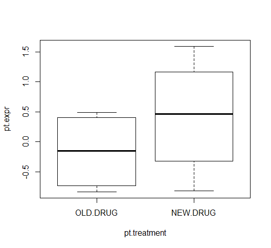
Factors help out when you want to either assess or plot the association between a treatment and a measured value (eg, the effect of the new drug on gene expression relative to the old drug). In the following the model equation "pt.expr ~ pt.treatment" tells R that you want to assess the effects of pt.treatment level on the variable pt.expr.

t.test(pt.expr ~ pt.treatment)

# various output: p.value = 0.11

# box-plot of the comparison

plot(pt.expr ~ pt.treatment)

You can use numeric, boolean or factor-variables on the right hand side of a model equation, but you can't use strings.

In the plot, the old-drug and new-drug are presented on the right- and left-hand sides, respectively. You'd normally plot the control group in the left-most region of a box plot, and in this imaginary experiment, it makes more sense for the old-drug to correspond to the control group. [Similarly, the t-test computes the difference OLD - NEW, rather than NEW - OLD]

R factors include a reference factor-level - it is the first factor level displayed by the function levels(), although you can also see this output following "Levels: " in the above:

levels(pt.sex)

# [1] "F" "M"

levels(pt.treatment)

# [1] "NEW.DRUG" "OLD.DRUG"

Note that alphabetically, "NEW.DRUG" < "OLD.DRUG" and "F" < "M".

R will always pick the alphanumerically-lowest value in a factor as its reference value, unless you explicitly tell it what the reference sample is. You can set the reference as follows:

pt.treatment <- factor(

rep(c("OLD.DRUG", "NEW.DRUG"), 4),

levels = c("OLD.DRUG", "NEW.DRUG")

)

pt.treatment

[1] OLD.DRUG NEW.DRUG OLD.DRUG NEW.DRUG OLD.DRUG NEW.DRUG OLD.DRUG

[8] NEW.DRUG

Levels: OLD.DRUG NEW.DRUG

plot(pt.expr ~ pt.treatment)

Matrices

Matrices are a 2-dimensional data structure containing n rows and m columns (for some integers n, m). Similarly to vectors, they can only store values of a single type. So you can have a matrix of numbers, or of strings, or of booleans, but not a combination of these types (if you combine numbers and strings in a matrix, the numbers will get converted into strings).

To construct a matrix, you can use the function matrix(data = some.data). This will work, provided you've previously defined a vector called some.data. By default, matrix(), will make a matrix with 1 column and as many rows as necessary to house the data that you provide. By changing the values of ncol and nrow in the call to matrix(), you can change the dimensions of the returned matrix. For example, to make a 3 by 2 matrix (ie, one with 3 rows and 2 columns), you could do the following :

matrix.of.numbers <- matrix(
data = c(1, 4, 3, 6, pi, exp(1)),
nrow = 3,
ncol = 2
)
# (1 6 )
# (4 3.14...)
# (3 2.71...)

Note that this fills the first column of the matrix with the first 3 entries in the data. Alternatively, you can tell R to fill up 'rows-first' as follows:

other.matrix <- matrix(
data = c(1, 4, 3, 6, pi, exp(1)),
nrow = 3,
ncol = 2,
byrow = TRUE
)
# (1.0 4.0)
# (3.0 6.0)
# (3.14.. 2.71..)

You can:

Check if a variable is a matrix with is.matrix()

is.matrix(vector.of.integers) # FALSE

is.matrix(matrix.of.numbers) # TRUE

Extract the dimensions of a matrix (ie, the number of rows and columns) using dim(), nrow(), ncol()

dim(matrix.of.numbers) # (3, 2)

nrow(matrix.of.numbers) # 3

ncol(matrix.of.numbers) # 2

Transpose a matrix, so that the first column of the input matrix is the first row in the output matrix (etc)

t(matrix.of.numbers)

# (1 4.0 3.0 )

# (6 3.14.. 2.71..)

dim(t(matrix.of.numbers)) # (2, 3)

Pull out submatrices of a matrix using some.matrix[which.rows, which.cols], where which.rows and which.cols are vectors of integers

matrix.of.numbers[2, 1] # 4

matrix.of.numbers[1, 2] # 6

matrix.of.numbers[2:3, 1:2]

# (4 3.14..)

# (3 2.71..)

Pull out a whole row (some.matrix[which.row, ]), or a whole column (some.matrix[, which.col])

matrix.of.numbers[3, ] # (3.0, 2.71..)

matrix.of.numbers[, 2] # (6.0, 3.14.., 2.71..)

.. and similarly you can change the values stored in a particular row, a particular column or in a row/column pair (using some.matrix[which.rows, which.cols] <- some.replacement)

Note that in RNASeq and microarray analysis, respectively, the read counts and fluorescence intensities are stored in a large numeric matrix with a row for each gene/transcript/probe and a column for each sample - so manipulating matrices is pretty useful.

[The similarities between matrices and vectors runs quite deep, indeed you could view vectors as being matrices with a single column; but really the converse is true, R stores an n by m matrix as a vector of length nm with the first n entries in the vector being the first column of the matrix]

Data frames

The data.frame is a 2-dimensional data structure. You can store a variety of different data-types in a data.frame (unlike in matrices), the only constraint is that each column must contain data of the same type (since, internally, the columns of a data.frame are vectors). So a data.frame provides a similar structure to that used in more hands-on tools like SPSS or graphpad

Suppose we have ran a microarray experiment on a bunch of patient-derived samples. To store the patient-specific metadata for such an experiment - you might need three vectors containing

patient-identifiers (as a string);

the sex of the patients (as a factor); and

the age of the patients (as a numeric column).

Here, the three vectors are connected in some way: the first entry in each corresponds to the first patient, the second entry to the second patient (etc). This representation is a bit inefficient, since if one of the patients is subsequently dropped from the experiment, you'd have to change three different vectors independently. By encapsulating these vectors in a data.frame you alleviate this inefficiency.

metadata <- data.frame(
id = c("A123", "B346", "C789"),
sex = factor(c("M", "F", NA)),
age = c(60, 62, 78),
stringsAsFactors = FALSE
)
# id sex age
# 1 A123 M 60
# 2 B346 F 62
# 3 C789 <NA> 78

# drop the third sample
# - you could also use metadata[-3, ]
new.metadata <- metadata[1:2, ]
# id sex age
# 1 A123 M 60
# 2 B346 F 62

To find out what type of data is stored in each column you can use the str() function:
str(metadata)
# 'data.frame': 3 obs. of 3 variables:
# $ id : chr "A123" "B346" "C789"
# $ sex: Factor w/ 2 levels "F","M": 2 1 NA
# $ age: num 60 62 78

Note that when we defined metadata, we used the argument stringsAsFactors = FALSE. The data.frame function is set up to automatically convert any string variables to factors, but here, the ID variable is not being used as a statistical factor, so we have to explicitly tell R not to convert it into a categorical variable. There are some occasions where treating patient or sample IDs as a factor is necessary - for example, if multiple samples from the same individual are present in an experiment, you can include the patient ID as a matching factor.

Many of the functions that act on data.frames are similar to those for matrices:

metadata[which.rows, which.cols] for subsetting

.. and metadata[which.rows, which.cols] <- some.replacement

dim, nrow, ncol

is.data.frame

Indexing by row/column names

Bioconductor contains some specialised data structures for holding microarray (called an ExpressionSet) and RNASeq datasets. In addition to the large matrix of expression intensities or read-counts (mentioned above: rows = features; columns = samples), these typically contain:

a data.frame containing info about the samples (rows = samples; eg, the experimental treatments for the biological samples, the extraction protocol),
a data.frame containing info about the features (rows = features; eg, what gene, genomic position or sequence do the features correspond to; other functional annotations of those genes)
other meta-data regarding the microarray platform, the paper where the data was published etc etc

the rows of (1) and the rows of (2) correspond to the columns and rows of the expression matrix, respectively.

Above, we showed that you can use integers to index particular rows/columns of a data.frame/matrix and hence, either extract or modify the values that are currently stored in the data.frame/matrix. Additionally, you can provide names for the rows/columns and use these to subset a data.frame or matrix. In the expression matrix for a microarray experiment, you'd typically use the probe ids to label the rows, and unique sample ids to label the columns (and label the rows of (1) and (2) to match).

To add these labels you can use the rownames(), colnames() functions or you can define them at definition of a matrix/data.frame

An example:

pt.ids <- paste("pt", 1:8, sep = "")

# (pt1 pt2 pt3 pt4 ... pt8)

pt.df <- data.frame(

# colnames 'sex' and 'treatment' are added automatically

sex = pt.sex,

treatment = pt.treatment,

row.names = pt.ids

)

pt.exprs <- matrix(

pt.expr,

nrow = 1,

ncol = 8

)

colnames(pt.exprs) <- pt.ids

rownames(pt.exprs) <- "gene1"

pt.df

# sex treatment

# pt1 F OLD.DRUG

# pt2 F NEW.DRUG

# pt3 F OLD.DRUG

# pt4 F NEW.DRUG

# pt5 M OLD.DRUG

# pt6 M NEW.DRUG

# pt7 M OLD.DRUG

# pt8 M NEW.DRUG

pt.exprs

# pt1 pt2 pt3 pt4 pt5 pt6 pt7 pt8

# gene1 -0.6265 0.1836 -0.8356 1.595 0.3295 -0.8205 0.4874 0.7383

Then you can subset as follows:

pt.df[c("pt4", "pt6"), ]

pt.df[, "treatment"] # or pt.df$treatment

pt.exprs[, c("pt4", "pt6")]

pt.exprs["gene1", ]

This can make it a lot easier to pull out data that you're interested in when you've got thousands of genes and hundreds of samples in a dataset

Functions & Help

You've already used a range of functions, if you've typed in the code so far: demo, seq, is.vector, length, c, rep, factor, set.seed, rnorm, t.test, plot, levels, matrix, t, data.frame, etc etc. Suppose you didn't know what the seq function does, you can get its helppage up in R or RStudio by typing in
? seq
# or help("seq")

Functions do things. They might take some input, process it and return some value. For example, mean is a function that takes a vector of numbers and returns the mean of those numbers. Sometimes it might not be obvious that a function even returns a value, for plot and set.seed for example (their side effects are more important than their return value: plotting data and setting the random number generator).

But, for functions to do anything, you have to provide them the right input (aka arguments).

On Unix, there is a program called grep and when you provide it with a string and some filenames, it will read each file and print out any lines in those files that contain the string to the command line. grep has a namesake within R that does something very similar. In the right hands, grep is a fine function. Check out it's help page. You can also check what arguments it takes using args(grep) and/or formals(grep), or by looking at it's source code by typing grep (without any parentheses) or by just running it with no arguments and watching it break. Here's what I get:

args(grep)
# function (pattern, x,
# ignore.case = FALSE, perl = FALSE, value = FALSE,
# fixed = FALSE, useBytes = FALSE, invert = FALSE)
# NULL

There are 8 arguments to grep. You don't have to provide values for all of them arguments - for example, ignore.case is given a default value of FALSE, so if you don't give it an alternative value the function will still run. Evidently pattern and x are the only arguments that must be provided by the user (since they have no default value in the args). In R, you can provide arguments to functions by putting the values in the appropriate order:

# Positional matching:
# - R can work out that "AB*" is intended to be `pattern`
# - and c("abc", "ABC", "ABD") is intended to be `x`
grep("AB*", c("abc", "ABC", "ABD"))
# [1] 2 3

The function has found that the second and third elements of x match the provided pattern. Suppose you want to find the elements that don't match the pattern, from the helppage, you need to set invert to TRUE (what would setting value=TRUE do instead of changing invert?). To do this using positional matching, you'd have to set values for 8 different arguments. Instead, you can set the argument values using their names - all of the following forms can do the inverted match:

# positional (F/T are shorthand for FALSE/TRUE)
grep("AB*", c("abc", "ABC", "ABD"), F, F, F, F, F, T)

# positional for the first 2, by-name for invert
grep("AB*", c("abc", "ABC", "ABD"), invert = TRUE)

# by-name for all
grep(pattern = "AB*", x = c("abc", "ABC", "ABD"), invert = TRUE)

# by-name don't care about order
grep(invert = TRUE, pattern = "AB*", x = c("abc", "ABC", "ABD"))

grep, gsub, substr are quite powerful ways of manipulating and searching against strings; I find gsub particularly useful for working out what treatments were used in each sample in a microarray ExpressionSet.

Other functions you might find helpful are which, intersect, sort

You can write your own functions. This is particularly valuable if you find yourself writing the same code over and over. But we'll leave that for another day. The syntax is

function_name <- function(
arg1,
arg2,
arg3 = some.default.value
){
# <body of the function>
some.return.value
}

Packages

All the stuff we've done so far has only used functions that are available in the most basic R installation. Various packages are available that can extend R - for our microarray analysis work we only need pacakges available from CRAN (the comprehensive R archive network) and bioconductor (which houses tons of well-documented bioinformatics pacakges). To use these, you have to install them and then load them:

# To install the `ggplot2` package for statistical graphics from CRAN:
install.packages("ggplot2")

# To install the `limma` package for microarray analysis from bioconductor:
# - Note that source(some.file) reads in and runs the script "some.file"
# - The script biocLite.R reads in a function called `biocLite`
source("http://www.bioconductor.org/biocLite.R")
biocLite("limma")

You'll need a couple of other packages to get through the stuff later in the tutorial. So try and install the following: GEOquery (which allows you to download datasets from NCBI::GEO to your computer and use them in an R session) and gplots (which provides a tool to make heatmaps).

That's installation done. To actually load the packages you have to type
library("<package.name>")

So, get loading the packages you've just installed: ggplot2, limma, GEOquery and gplots.

Each of these packages provides a different bunch of functions and data structures that should make your life easier, or more beautiful. Basic R plots, like the Box-plots above, are OK and you can configure them to do a lot of cool stuff. You might find ggplot2 plots a bit prettier (the two main functions in ggplot2 are ggplot and qplot, the latter is a bit easier):

qplot(
x = pt.treatment,
y = pt.expr,
geom = "boxplot"
)

# equivalent:
dframe <- data.frame(
treatment = pt.treatment,
sex = pt.sex,
expr = pt.expr
)

ggplot(
data = dframe,
aes(x = treatment, y = expr)
) +
geom_boxplot()

Microarray analysis

You're going to

use GEOquery to download some microarray data from the Gene Expression Omnibus;
decide which bits of that dataset to use (which probes, which samples);
define a statistical model for that dataset in limma;
define an experimental contrast that you're interested in
identify some differentially expressed genes
plot out a heatmap and some other plots of the data

.. and hopefully your prior scientific knowledge and the code we've worked through above should get us through that workflow.

[There are some steps of microarray analysis that we won't touch on: normalising raw data, post-genomic stuff like GO enrichment, and we're going to keep the experimental designs as simple as possible]

Obtain data using GEOquery

I have recent experience with the following datasets: GSE47927, GSE11889, GSE43754, GSE5550
If you have another dataset that you're interested in you can use that, but otherwise, just pick one of the identifiers from the above, read the write up for the dataset at GEO to get an idea of what experimental comparisons have been performed. Then have a look at the GEOquery vignette, especially section 4.1.

The function getGEO can download your chosen dataset. It will save the dataset locally on your computer and then read the relevant files into your R session. You'd use a call similar to:

# - Might take a few minutes ...
# - Don't worry if you get the warning "not all columns named in 'colClasses' exist"
# Download and import a microarray series from NCBI::GEO
gse.series <- getGEO(
GEO = "<fill in>",
destdir = "<the blanks>"
)

If this works it will store your dataset in the variable gse.series. I normally store the downloaded datasets in the directory "~/ext_data/GEOquery/" [on unix] or "C://ext_data/GEOquery/" [on windows]. If you don't provide a destination directory, the data will be stored in a temporary folder and deleted after your session has closed.

To quote the GEOquery vignette: "The data structure returned from this parsing is a list of ExpressionSets". ExpressionSets were mentioned above, but we haven't mentioned lists. Lists are a more versatile data structure than vectors, matrices or data.frames - they are one-dimensional like vectors but can store distinct datatypes, and you can access their elements like so: some.list[[some.index]] or some.list$some.label.

All you need to know at this stage is that gse.series is a list, and if you've picked one of the GSE-ids above there'll only be one element in that list - the ExpressionSet that we're going to analyse. We can pull that ExpressionSet out as follows:

gse <- gse.series[[1]]

[If you really want, you can obtain the raw data from a microarray dataset using GEOquery's getGEOSuppFiles function and do all the array normalisation stuff yourself; but the datasets I've picked out have already been normalised]

[Similar functions are available for datasets stored at ArrayExpress: see the bioconductor::arrayExpress package; later try running this whole thing on one of their datasets - like E-MTAB-2581 - although to analyse that dataset you'll need to know about reading in raw microarray CEL files and array normalisation - see the affy or oligo packages]

Filter the dataset

The ExpressionSet stored in gse might be pretty complicated. This will print out a summary of the dataset:

gse
# ExpressionSet (storageMode: lockedEnvironment)
# assayData: 232479 features, 20 samples
# element names: exprs
# protocolData: none
# phenoData
# sampleNames: <names of the samples> (20 total)
# varLabels: <info about the samples>
# varMetadata: <info about the samples>
# featureData
# featureNames: <names of the microarray probes> (232479 total)
# fvarLabels: <info about the probes>
# fvarMetadata: <info about the probes>
# experimentData: use 'experimentData(object)'

# Annotation: <some microarray platform>

You can access

the data.frame containing info about the samples using pData(gse)
the data.frame containing info about the probes using fData(gse)
the matrix of microarray intensities using exprs(gse)

Before proceeding, you should check if the microarray data are log-transformed - a histogram of the intensities will look approximately normally distributed if they are:

# A histogram of the microarray log-intensities across all samples

hist(x = <fill in the blank>)

So that the analysis is easy, we'll restrict to just a single experimental contrast. In the datasets suggested above, there are a number of possible contrasts:

stem vs progenitor in CML
stem vs progenitor in Normal
CML-stem vs Normal-stem
CML-progenitor vs Normal-progenitor
Chronic-phase stem cells vs accelerated-phase stem cells
etc etc etc

Determine what comparisons you can do with the dataset that you have downloaded (based on the metadata at GEO) and pick one of those comparisons for follow-up. In GSE43754, you could do stem vs progenitor in non-CML individuals (hopefully you've picked a different comparison) - the initial dataset contains 20 samples, we restrict to just the normal samples.

# The data.frame pData(gse) contains the sample-specific info

names(pData(gse))

# - to restrict to normal samples, I have to find them first:

# - 'title' and 'characteristics_*' columns usually help

# - recall how to subset a data.frame:

cols <- c("title", "characteristics_ch1",

"characteristics_ch1.1", "characteristics_ch1.2")

pData(gse)[, cols]

The column "characteristics.ch1.1" indicates the disease state of the samples (either "disease state: Normal" or "disease state: chronic myeloid leukemia"). To identify the normal samples I could use the following

keep.samples <- grep(

pattern = "Normal",

x = pData(gse)$characteristics_ch1.1

)

# or equivalently:

# keep.samples <- which(

# pData(gse)$characteristics_ch1.1 == "disease state: Normal"

# )

To restrict to just these samples is really easy. The heart of the ExpressionSet is the matrix of expression intensities and it's indexed by probes (along the rows) and samples (along the columns). Just as you'd subset a matrix using some.matrix[, which.cols], you can subset an ExpressionSet using some.eset[, which.samples] (or some.eset[which.probes, ] if you wanted to restrict the probes that you analyse). If you restrict an expression set this way, the featureData, exprs, phenoData are all automatically updated to refer to just those samples that remain.

# restrict to just my samples of interest (just the normal samples)

new.gse <- gse[, keep.samples]

new.gse

# blah blah (10 samples)

Try and work out how to restrict your gse to just those samples that are relevant to your experimental comparison - again using grep to find the appropriate indices of the samples you want to keep.

[I wouldn't normally restrict the samples in this way, but it simplifies the tutorial. I'd normally include all the different experimental arms throughout the statistical modelling, and only perform a statistical contrast for normal_stem minus normal_progenitor samples]

Define the statistical model

Again this section depends upon the dataset that you've downloaded and the experimental contrast that you've chosen to analyse.

Before you can run limma and assess differential expression, you have to encode the different experimental arms that are present in your dataset. For my comparison, I therefore have to encode which of the samples are Stem-cells, and which samples are Progenitor-cells (remember they're all from non-CML individuals, so I don't have to also encode CML vs Normal).

Again this information is contained in pData (for the dataset I'm using it's all in characteristics_ch1.2). This time you'd want to convert the info into a factor though (see above).

celltype <- pData(new.gse)[, 'characteristics_ch1.2']
head(celltype)
# V4 V5
#cell type: normal progenitor cell type: normal progenitor
# V9 V10
#cell type: normal progenitor cell type: normal progenitor
# V11 V14
#cell type: normal progenitor cell type: normal stem
#4 Levels: cell type: chronic myeloid leukemia progenitor ...

Err no! it already is a factor, and it contains levels that no longer exist. Let's just redefine it. Remember I mentioned gsub. The syntax is similar to grep, but this time anything that matches pattern is replaced with replacement. See how the values of celltype all start "cell type: normal ...". Let's drop that (you shouldn't have any spaces in your factor levels after this point anyway):

celltype <- gsub(
pattern = "cell type: normal ",
replacement = "",
x = celltype
)
head(celltype)
# [1] "progenitor" "progenitor" "progenitor" ... "stem" "stem"

To convert that to a factor, taking "progenitor" as reference:
celltype <- factor(celltype, levels = c("progenitor", "stem"))

We can now use celltype in model equations. You use model equations to define a model.matrix that limma uses to best-fit a bunch of coefficients (here we've set it up to fit a coefficient for progenitors and a coefficient for stemcells):
design.mat <- model.matrix(~ -1 + celltype)
design.mat
# compare model.matrix(~ celltype) and model.matrix(~ -1 + celltype)
# - they're the same underlying model, but they're parametrized differently
# we rename the columns for clarity
colnames(design.mat) <- levels(celltype)

Again, work out how to encode your experimental factors into a design matrix - use the pData to find which samples map to which treatments, make a factor, convert it into a design matrix using model.matrix

[You can actually define celltype in one step:
# celltype <- factor(
# gsub(
# pattern = "cell type: normal ", replacement = "",
# x = pData(new.gse)[, 'characteristics_ch1.2']
# ),
# levels = c("progenitor", "stem"))
#
# Or, my favourite
# library(magrittr) # imports an operator %>%
#
# celltype <- pData(new.gse)[, 'characteristics_ch1.2'] %>%
# gsub(pattern = "cell type: normal ",
# replacement = "",
# x = .) %>%
# factor(levels = c("progenitor", "stem"))
]

Define the experimental contrast

Once limma has fitted the coefficients (one for each column in design), you can use their estimates in hypothesis tests, but you have to tell limma what hypothesis you want to test. Here we want to test against the null hypothesis that for a given probe, the intensity in stemcells and progenitor cells is the same, that is, that there should be no difference between the coefficient for "progenitor" and that for "stem".

contrasts.mat <- makeContrasts(
stem.v.prog = "stem - progenitor",
levels = design.mat
)
contrasts.mat

Identify differentially detected probes

Obtaining and filtering the data, defining the experimental design and the experimental contrasts are now done. All you have to do is run your data/design through the limma workflow (this is all covered in a load of detail in the limma user's guide). The steps are as follows:

# estimate the design coefficients

fit.lm <- lmFit(new.gse, design.mat)

# estimate the contrast coefficients

fit.cont <- contrasts.fit(fit.lm, contrasts.mat)

# regularise the contrast coefficients

fit.eb <- eBayes(fit.cont)

topTable(fit.eb) # most differentially expressed probes

summary(decideTests(fit.eb)) # number of diffexes

Plot out some data

tt <- topTable(fit.eb, n = Inf)

plot(logFC ~ AveExpr, data = tt, pch = '.')

# TODO - heatmap.2

biolearnr

Thursday 9 February 2017

Start playing with R and Bioconductor